SQL in Fusion 3

In this post, I introduce a new service in Fusion  that allows users to execute SQL queries against their Fusion collections using any JDBC compliant application, such as Tableau or Apache Zeppelin. Before diving into the details of how to use the SQL service, let’s first understand why Lucidworks is excited to offer this new feature.

Motivation

One of the patterns we see with our customers is that they use Fusion to solve a search problem but then quickly realize they have a big data problem in that they can now capture user-generated events, known as signals in Fusion, from the search application. This is a good problem to have, as these signals can be fed back into the search experience in the form of relevancy boosting, recommendations, and other machine learning models, such as query intent classification. These signals are also a veritable goldmine of semi-structured information about your users and the Fusion SQL service provides new opportunities for analyzing this data using BI tools like Tableau.

Self-service Analytics

Providing self-service analytics solutions ranks high on the priority list for many CIOs, especially when it comes to big data projects, as data scientists and big data engineers are scarce resources. Moreover, SQL remains the lingua-franca of analytics and there are many data visualization and dashboarding tools that support SQL. With the release of Fusion 3, business analysts can discover, analyze, and visualize datasets of interest using their SQL tool of choice. This eliminates retraining users on proprietary tools and query languages, which increases return on investments made in visualization tools.

What good is self-service if the data is locked in silos? Fusion provides connectors for indexing data from 60+ enterprise systems and databases. Ultimately, numerous mission-critical data sets work their way into Fusion because of the speed, flexibility, and scalability of Solr. The SQL service exposes Solr’s capabilities including relevancy ranking of documents, fuzzy free-text search, graph traversals across relationships, and on-the-fly application of classification and machine learning models for these mission critical data sets.

In most organizations, there are subject matter experts (SME) for specific datasets. The Fusion SQL service provides SMEs a way to leverage their expertise in the form of data transformations, enrichments, and filtering while hiding complexity from other consumers of a shared dataset. For instance, a data engineer working with the support organization can use Fusion to expose a view for the marketing and sales teams to help them understand current customer support issues. Being able to create “views” of complex data sources is especially important for organizations with a data lake, where the source data may be messy and require a number of transformations in order to be useful to business analysts. Although the SQL engine is powered by massively scalable technologies like Apache Spark and Apache Solr, the business analyst doesn’t need to reason about these complex technologies and can stay focused on asking the important questions from their data.

Deeper Analytic Capabilities

Up to this point, Fusion’s analytics story has centered around visualizing facet queries on data stored in Solr. With the SQL service, we now can go beyond facet queries to perform more advanced analytics, such as powerful SQL aggregations using a wealth of built-in UDF/UDAF functions, multi-dimensional OLAP cubes, and joins across multiple Solr collections and/or external data sources (Hive table, Cassandra CF, JDBC database, etc).

Also, the common prescription to denormalize data for fast ranked retrieval in Solr is not always practical/possible for analytical type use cases. Consequently, Fusion’s SQL service gives users the ability to join across tables.

Data Governance

Lastly, data governance, especially for big data, continues to be a major concern for CIOs. The SQL service uses Fusion permissions to guard access to sensitive datasets, giving Fusion administrators full control over which tables a user can query.

At this point, I hope I gave you a few reasons to be excited about the SQL service in Fusion. Next, let’s kick the tires on the engine to see how it works.

Getting Started

If you haven’t done so already, please download and install Fusion from: lucidworks.com/download
For this blog, we’ll use $FUSION_HOME to represent the directory where you installed Fusion, such as: /opt/fusion/3.0.0.

Start Fusion if it is not running:

cd $FUSION_HOME
bin/fusion start

Login to the Fusion Admin UI at: http://localhost:8764/

You should also start the Fusion SQL service by doing:

bin/sql start

You can jump right in and start using the SQL service with your own data, but for instructional purposes, I’ll walk you through the movielens lab in our fusion-spark-bootcamp project. The movielens dataset is a good example for the SQL service because it has multiple tables we can join across, full-text fields, and geo-spatial data.

Open a command-line terminal and clone the github project by doing:

git clone https://github.com/lucidworks/fusion-spark-bootcamp.git

Tip: If you’re not a git user, no problem you can download the project zip file from fusion-spark-bootcamp/master.zip.

cd fusion-spark-bootcamp

Edit the myenv.sh script to set the variables for your environment.

cd labs/movielens
./setup_movielens.sh

The setup script will download the movielens dataset and load it into Fusion. It may take a couple of minutes to run the first time as the Fusion spark-shell wrapper script needs to download the Fusion job jar for Spark jobs. After the setup script completes, you will have the following tables available to query via SQL:

To verify the SQL engine is running and the movielens tables are loaded correctly, you can do:

curl -XPOST -H "Content-Type:application/json" 
"http://localhost:8765/api/v1/catalog/fusion/query" -d '{"sql":"show tables"}'

Also, the movielens lab includes an explore_movielens.sh script that uses the Fusion Catalog API to explore the dataset and execute SQL statements. The Catalog API is a higher level API that uses JDBC to send queries and manage data assets in the SQL engine. For more information about the Catalog API, see:
REST_API_Reference/Catalog-API.html

JDBC Connectivity

In the next section, I’ll use Tableau to explore the movielens dataset. If you don’t have Tableau available, you can use any client application that supports JDBC. A good open source option is Apache Zeppelin, which we’ll blog about in the near future. Here are the settings if you want to use JDBC to access the SQL service:

Driver: org.apache.hive.jdbc.HiveDriver
URL: jdbc:hive2://:8768/default?hive.server2.transport.mode=http;hive.server2.thrift.http.path=fusion

The username and password will be the same you use to authenticate to Fusion.

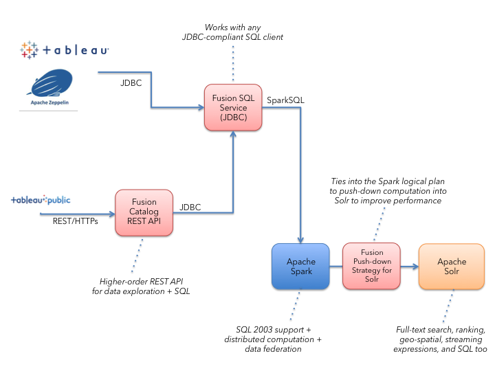
The following diagram depicts the SQL engine architecture so you can see where tools like Tableau and the Catalog API fit:

Connecting to Fusion’s SQL Service from Tableau

I chose to use Tableau for this blog as it produces beautiful visualizations with little effort and is widely deployed across many organizations. I provide instructions for connecting with Tableau Desktop Professional and Tableau Public.

Tableau Desktop Professional

If you have the professional version of Tableau Desktop, then you can use the Spark SQL connector; you may have to install the Spark SQL driver for Tableau, see https://onlinehelp.tableau.com/current/pro/desktop/en-us/examples_sparksql.html and https://databricks.com/spark/odbc-driver-download

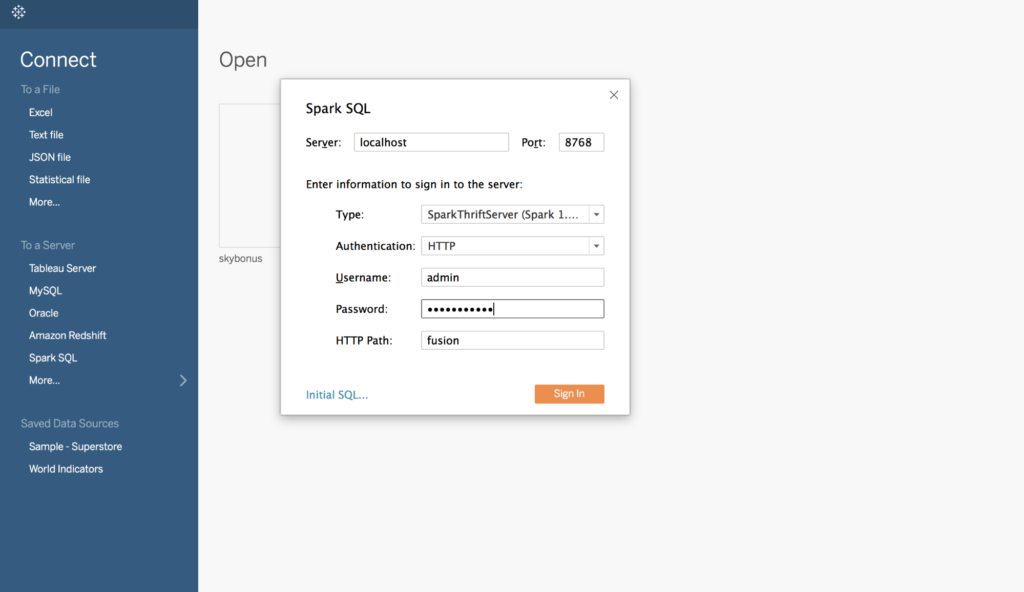
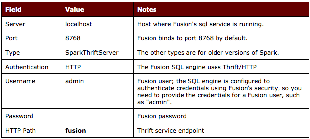
Fill in the Spark SQL connection properties as follows:

Once connected, you need to select the “default” schema as illustrated in the following screenshot.

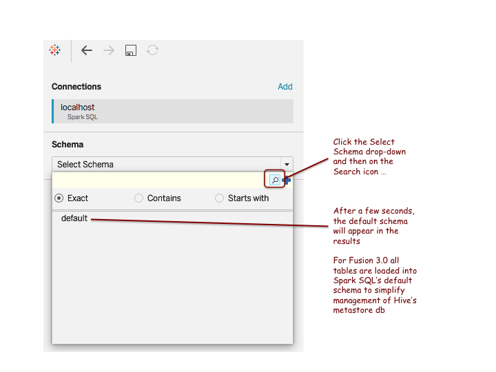
After selecting the default schema, click on the search icon to show all tables / views registered in the SQL engine by the Fusion Catalog.

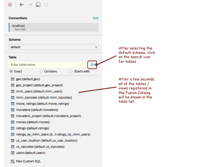
Note: you may see a different list of tables than what is shown in this illustrative screenshot.

Fusion Web Data Connector with Tableau Public

If you don’t have access to the professional version of Tableau Desktop, you can use the experimental (not officially supported) beta version of Fusion’s Web Data Connector (WDC) for Tableau and/or Tableau Public. The WDC has limited functionality compared to the professional desktop version (it’s free), but is useful for getting started with the Fusion SQL engine.

Open a terminal and clone the following project from github:

git clone https://github.com/lucidworks/tableau-fusion-wdc.git

After cloning the repo, cd into the tableau-fusion-wdc directory and do:

npm install --production
npm start

You now have a web server and cors proxy running on ports 8888 and 8889 respectively.

For reference see: http://tableau.github.io/tableau-fusion-wdc/docs/

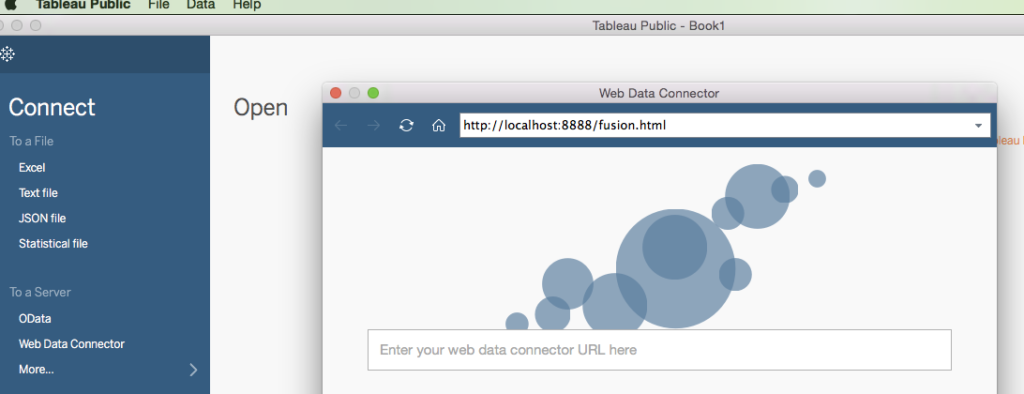
Download, install, and launch Tableau Public from: https://public.tableau.com/en-us/s/download

Click on the Web Data Connector link under Connect and enter: http://localhost:8888/fusion.html as shown below:

In the Fusion dialog, click on the Load Fusion Tables button:

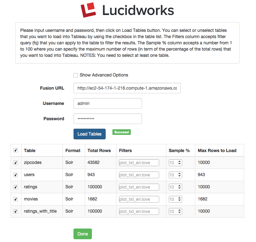
Note: The list of tables you see may be different than what is shown in the example screenshot above.

Select the tables you want to import and optionally apply filters and/or sampling. For small tables (<50K rows), you don’t need to filter or sample. Click Done when you’re ready to load the tables into Tableau Public. After a few seconds, you should see you tables listed on the left.

Note: only Fusion collections that have data are shown. If you add data to a previously empty collection, then you’ll need to refresh Tableau Public to pick it up.

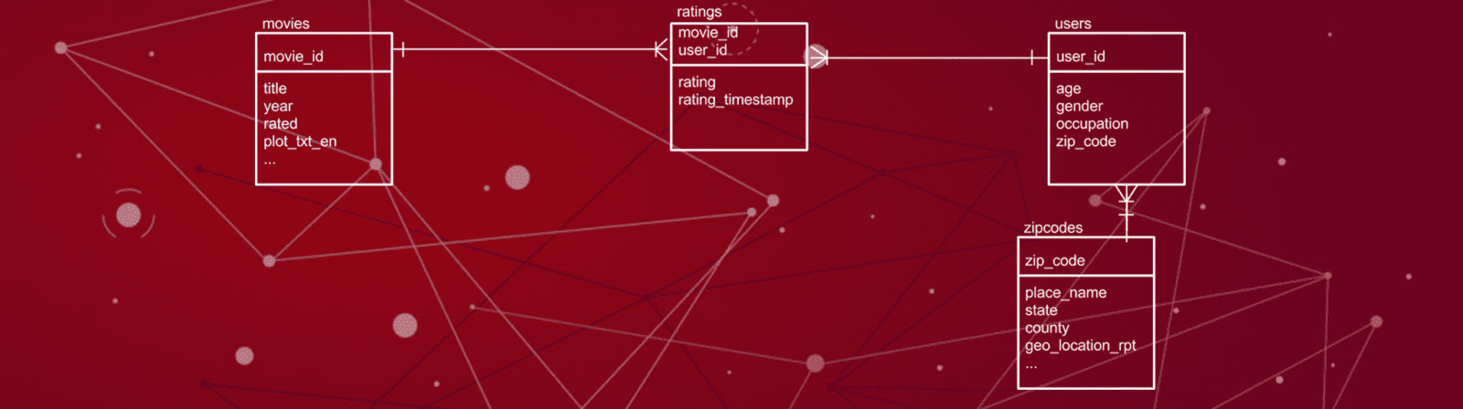
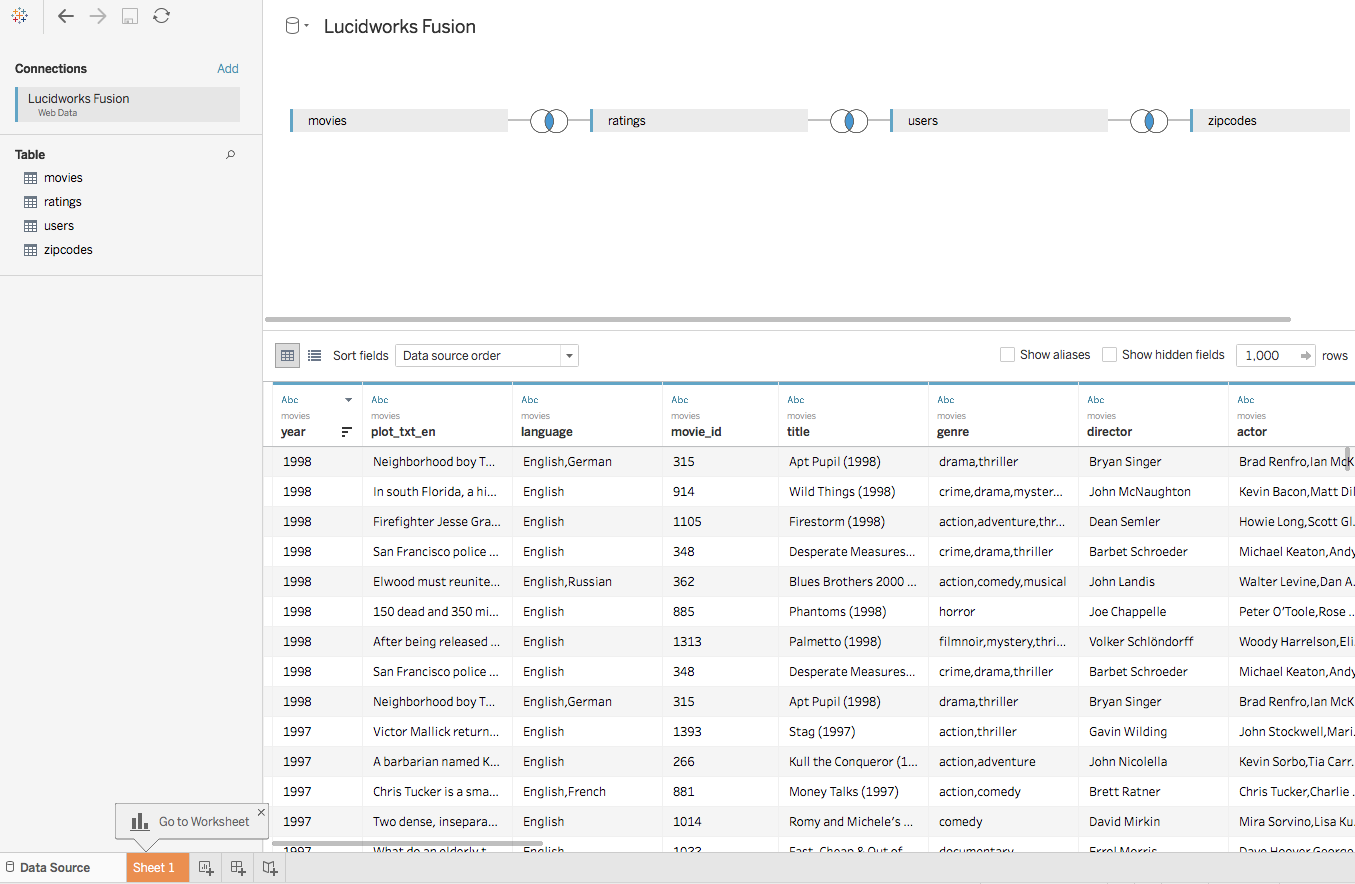
Let’s create a Tableau Data Source that joins the 4 tables (movies, ratings, users, and zipcodes) together as shown below:

Next, click on the Sheet 1 button and build a visualization with our data from Fusion. Note that Tableau Public builds an extract of your dataset and pulls it down to the desktop before applying any filters. Consequently, be careful with large tables; use the filter options on the initial Fusion WDC screen to limit data. The professional version sends queries back to the Fusion SQL engine and as such can handle larger datasets more efficiently.

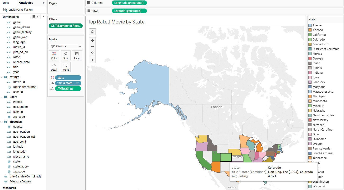
Here’s a visualization where I used a nested sort to find the most liked movie by state (using avg rating):

Here are a few SQL queries for the movielens dataset to help get you started:

Aggregate then Join:

SELECT m.title as title, solr.aggCount as aggCount FROM movies m INNER JOIN (SELECT movie_id, COUNT(*) as aggCount FROM ratings WHERE rating >= 4 GROUP BY movie_id ORDER BY aggCount desc LIMIT 10) as solr ON solr.movie_id = m.movie_id ORDER BY aggCount DESC

Users within 50 km of Minneapolis:

SELECT solr.place_name, count(*) as cnt FROM users u INNER JOIN (select place_name,zip_code from zipcodes where _query_='{!geofilt sfield=geo_location pt=44.9609,-93.2642 d=50}') as solr ON solr.zip_code = u.zip_code WHERE u.gender='F' GROUP BY solr.place_name

Avg. Rating for Movies with term “love” in the Plot:

SELECT solr.title as title, avg(rating) as avg_rating FROM ratings INNER JOIN (select movie_id,title from movies where _query_='plot_txt_en:love') as solr ON ratings.movie_id = solr.movie_id GROUP BY title ORDER BY avg_rating DESC LIMIT 10

What types of cool visualizations can you come up with for the movielens or your data?

Tips and Tricks

In this section, I provide tips on how to get the best performance out of the SQL engine. In general, there are three classes of queries supported by the engine:

• Read a set of raw rows from Solr and join / aggregate in Spark
• Push-down aggregation queries into Solr, returning a smaller set of aggregated rows to Spark
• Views that send queries (Solr SQL or streaming expressions) directly to Solr using options supported by the spark-solr library

Aggregate in Spark

For queries that rely on Spark performing joins and aggregations on raw rows read from Solr, your goal is to minimize the number of rows read from Solr and achieve the best read performance of those rows. Here are some strategies for achieving these goals:

Strategy 1: Optimal read performance is achieved by only requesting fields that have docValues enabled as these can be pulled through the /export handler

It goes without saying that you should only request the fields you need for each query. Spark’s query planner will push the field list down into Fusion’s SQL engine which translates it into an fl parameter. For example, if you need movie_id and title from the movies table, do this:

select movie_id, title from movies

Not this:

select * from movies

Strategy 2: Use WHERE clause criteria, including full Solr queries, to do as much filtering in Solr as possible to reduce the number of rows

Spark’s SQL query planner will push down simple filter criteria into the Fusion SQL engine, which translates SQL filters into Solr filter query (fq) parameters. For instance, if you want to query using SQL:

select user_id, movie_id, rating from ratings where rating = 4

Then behind the scenes, Fusion’s SQL engine transforms this query into the following Solr query:

q=*:*&qt=/export&sort=id+asc&collection=ratings&fl=user_id,movie_id,rating&fq=rating:4

Notice that the WHERE clause was translated into an fq and the specific fields needed for the query are sent along in the fl parameter. Also notice, that Fusion’s SQL engine will use the /export handler if all the fields requested have docValues enabled. This makes a big difference in performance.

To perform full-text searches, you need to use the _query_ syntax supported by Solr’s Parallel SQL engine, such as:

select movie_id,title from movies where _query_='plot_txt_en:love'

The Fusion SQL engine understands the _query_ syntax to indicate this query should be pushed down into Solr’s Parallel SQL engine directly. For more information about Solr’s Parallel SQL support, see: Solr’s Parallel SQL Interface. The key takeaway is that if you need Solr to execute a query beyond basic filter logic, then you need to use the _query_ syntax.

Here’s another example where we push-down a subquery into Solr directly to apply a geo-spatial filter and then join the resulting rows with another table:

SELECT solr.place_name, count(*) as cnt 
  FROM users u 
  INNER JOIN (select place_name,zip_code from zipcodes where _query_='{!geofilt sfield=geo_location pt=44.9609,-93.2642 d=50}') as solr 
  ON solr.zip_code = u.zip_code WHERE u.gender='F' GROUP BY solr.place_name

Notice that you need to alias the sub-query “as solr” in order for the Fusion SQL engine to know to perform the push-down into Solr. This limitation will be relaxed in a future version of Fusion.

Strategy 3: Apply limit clauses on push-down queries

Let’s say we have a table of movies and ratings and want to join the title with the ratings table to get the top 100 movies with the most ratings using something like this:

select m.title, count(*) as num_ratings from movies m, ratings r where m.movie_id = r.movie_id group by m.title order by num_ratings desc limit 100

Given that LIMIT clause, you might think this query will be very fast because you’re only asking for 100 rows. However, if the ratings table is big (as is typically the case), then Spark has to read all of the ratings from Solr before joining and aggregating. The better approach is to push the LIMIT down into Solr and then join from the smaller result set.

select m.title, solr.num_ratings from movies m inner join (select movie_id, count(*) as num_ratings from ratings group by movie_id order by num_ratings desc limit 100) as solr on m.movie_id = solr.movie_id order by num_ratings desc

Notice the limit is now on the sub-query that gets run directly by Solr. You should use this strategy whether you’re aggregating in Solr or just retrieving raw rows, such as:

SELECT e.id, e.name, solr.* FROM ecommerce e INNER JOIN (select timestamp_tdt, query_s, filters_s, type_s, user_id_s, doc_id_s from ecommerce_signals order by timestamp_tdt desc limit 50000) as solr ON solr.doc_id_s = e.id

The sub-query pulls the last 50,000 signals from Solr before joining with the ecommerce table.

Strategy 4: When you need to return fields from Solr that don’t support docValues, consider tuning the read options of the underlying data asset in Fusion

Behind the scenes, the Fusion SQL engine uses parallel queries to each shard and cursorMark to page through all documents in each shard. This approach, while efficient, is not as fast as reading from the /export handler. For instance, our ecommerce table contains text fields that can’t be exported using docValues, so we can tune the read performance using the Catalog API:

curl -X PUT -H "Content-type:application/json" --data-binary '{
  "name": "ecommerce",
  "assetType": "table",
  "projectId": "fusion",
  "description": "ecommerce demo data",
  "tags": ["fusion"],
  "format": "solr",
  "cacheOnLoad": false,
  "options" : [ "collection -> ecommerce", "splits_per_shard -> 4", "solr.params -> sort=id asc", "exclude_fields -> _lw_*,_raw_content_", "rows -> 10000" ]
}' $FUSION_API/catalog/fusion/assets/ecommerce

Notice in this case, that we’re reading all fields except those matching the patterns in the exclude_fields option. We’ve also increased the number of rows read per paging request to 10,000 and want 4 splits_per_shard, which means we’ll use 4 tasks per shard to read data across all replicas of that shard. For more information on tuning read performance, see: spark-solr. The key take-away here is that if your queries need fields that can’t be exported, then you’ll need to do some manual tuning of the options on the data asset to get optimal performance.

Aggregate in Solr

Solr is an amazing distributed aggregation engine, which you should try to leverage as much as possible as this distributes the computation of aggregations and reduces the number of rows that are returned from Solr to Spark. The smaller the number of rows returned from Solr allows Spark to perform better query optimization, such as doing a broadcast of a small table across all partitions of a large table (hash join).

Strategy 5: Do aggregations in Solr using Parallel SQL

Here is an example where we push a group count operation (a facet basically) down into Solr using a sub-query.

    SELECT m.title as title, solr.aggCount as aggCount 
      FROM movies m 
INNER JOIN (SELECT movie_id, COUNT(*) as aggCount FROM ratings WHERE rating >= 4 GROUP BY movie_id ORDER BY aggCount desc LIMIT 10) as solr
        ON solr.movie_id = m.movie_id
  ORDER BY aggCount DESC

Solr returns aggregated rows by movie_id and then we leverage Spark to perform the join between movies and the aggregated results of the sub-query, which it can do quickly using a hash join with a broadcast. Aggregating and then joining is a common pattern in SQL, see:
use-subqueries-to-count-distinct-50x-faster.

Strategy 6: Aggregate in Solr using streaming expressions

Solr’s Parallel SQL support is evolving and does not yet provide a way to leverage all of Solr’s aggregation capabilities. However, you can write a Solr streaming expression and then expose that as a “view” in the Fusion SQL engine. For example, the following streaming expression joins ecommerce products and signals:

select(
  hashJoin(
    search(ecommerce,
           q="*:*",
           fl="id,name",
           sort="id asc",
           qt="/export",
          partitionKeys="id"),
    hashed=facet(ecommerce_signals,
                 q="*:*",
                 buckets="doc_id_s",
                 bucketSizeLimit=10000,
                 bucketSorts="count(*) desc",
                 count(*)),
    on="id=doc_id_s"),
  name as product_name,
  count(*) as click_count,
  id as product_id
)

This streaming expression performs a hashJoin between the ecommerce table and the results of a facet expression on the signals collection. We also use the select expression decorator to return human-friendly field names. For more information on how to write streaming expressions, see: Solr Streaming Expressions

Here’s another example of a streaming expression that leverages the underlying facet engine’s support for computing aggregations beyond just a count:

select(
  facet(
    ratings,
    q="*:*",
    buckets="rating",
    bucketSorts="count(*) desc",
    bucketSizeLimit=100,
    count(*),
    sum(rating),
    min(rating),
    max(rating),
    avg(rating)
  ),
  rating,
  count(*) as the_count,
  sum(rating) as the_sum,
  min(rating) as the_min,
  max(rating) as the_max,
  avg(rating) as the_avg
)

You’ll need to use the Catalog API to create a data asset that executes your streaming expression. For example:

curl -XPOST -H "Content-Type:application/json" --data-binary '{
  "name": "ecomm_popular_docs",
  "assetType": "table",
  "projectId": "fusion",
  "description": "Join product name with facet counts of docs in signals",
  "tags": ["ecommerce"],
  "format": "solr",
  "cacheOnLoad": true,
  "options": ["collection -> ecommerce", "expr -> select(hashJoin(search(ecommerce,q="*:*",fl="id,name",sort="id asc",qt="/export",partitionKeys="id"),hashed=facet(ecommerce_signals,q="*:*",buckets="doc_id_s",bucketSizeLimit=10000,bucketSorts="count(*) desc",count(*)),on="id=doc_id_s"),name as product_name,count(*) as click_count,id as product_id)"]}' $FUSION_API/catalog/fusion/assets

Strategy 7: Use sampling

With Fusion 3 and later, you’ll have to define a view backed to get a random sample of documents as the Parallel SQL implementation in Solr does not yet support random sampling. You’ll need to use the sample_pct option when reading from Solr:

{
  "name": "sampled_ratings",
  "assetType": "table",
  "projectId": "fusion",
  "description": "movie ratings data",
  "tags": ["movies"],
  "format": "solr",
  "cacheOnLoad": true,
  "options": ["collection -> movielens_ratings", "sample_pct -> 0.1", "sample_seed -> 5150", "fields -> user_id,movie_id,rating,rating_timestamp", "solr.params -> sort=id asc"]
}

NOTE: There is a random streaming expression decorator, but due to a bug, it was not exposed correctly until Solr 6.4, see: SOLR-9919

Strategy 8: Cache results in Spark if you plan to perform additional queries against the results

Catalog assets support the cacheOnLoad attribute which caches the results of the query in Spark (memory with spill to disk). You can also request the results for any query sent to the Catalog API to be cached using the cacheResultsAs param:

curl -XPOST -H "Content-Type:application/json" -d '{
  "sql":"SELECT u.user_id as user_id, age, gender, occupation, place_name, county, state, zip_code, geo_location_rpt, title, movie_id, rating, rating_timestamp FROM minn_users u INNER JOIN movie_ratings m ON u.user_id = m.user_id",
  "cacheResultsAs": "ratings_by_minn_users"
}' "$FUSION_API/catalog/fusion/query"

Be careful! If cached, updates to the underlying data source, most likely Solr, will no longer be visible. To trigger Spark to re-compute a cached view by going back to the underlying store, you can use the following SQL command:

curl -XPOST -H "Content-Type:application/json" -d '{"sql":"refresh table"}' "$FUSION_API/catalog/fusion/query"

If a table isn’t cached, you can cache it using:

curl -XPOST -H "Content-Type:application/json" -d '{"sql":"cache table"}' "$FUSION_API/catalog/fusion/query"

Or uncache it:

curl -XPOST -H "Content-Type:application/json" -d '{"sql":"uncache table"}' "$FUSION_API/catalog/fusion/query"

Strategy 9: Use SQL and Spark’s User Defined Functions (UDF) to clean and/or transform data from Solr

For example, the search hub signals use complex field names generated by snowplow. The following data asset definition uses SQL to make the data a bit more user friendly as it comes out of Solr:

{
  "name": "shub_signals",
  "assetType": "table",
  "projectId": "fusion",
  "description": "SearchHub signals",
  "tags": ["shub"],
  "format": "solr",
  "cacheOnLoad": false,
  "options": ["collection -> shub_signals", "solr.params -> sort=id asc", "fields -> timestamp_tdt,type_s,params.useragent_family_s,params.useragent_os_family_s,params.tz_s,params.totalResults_s,params.lang_s,params.useragent_type_name_s,params.terms_s,params.query_unique_id,params.useragent_v,params.doc_0,params.doc_1,params.doc_2,params.facet_ranges_publishedOnDate_before_d,params.uid_s,params.refr_s,params.useragent_category_s,params.sid_s,ip_sha_s,params.vid_s,params.page_s,params.fp_s"],
  "sql": "SELECT timestamp_tdt as timestamp, type_s as signal_type, `params.useragent_family_s` as ua_family,`params.useragent_os_family_s` as ua_os,`params.tz_s` as tz,cast(`params.totalResults_s` as int) as num_found, `params.lang_s` as lang, `params.useragent_type_name_s` as ua_type, `params.terms_s` as query_terms, `params.query_unique_id` as query_id, `params.useragent_v` as ua_vers, `params.doc_0` as doc0, `params.doc_1` as doc1, `params.doc_2` as doc2, `params.facet_ranges_publishedOnDate_before_d` as pubdate_range, `params.uid_s` as user_id, `params.refr_s` as referrer, `params.useragent_category_s` as ua_category, `params.sid_s` as session_id, `ip_sha_s` as ip, cast(`params.vid_s` as int) as num_visits, `params.page_s` as page_name, `params.fp_s` as fingerprint FROM shub_signals"
}

Given how Spark uses lazy evaluation of DataFrame transformations, there is little additional overhead beyond the cost of reading from Solr to execute a SQL statement on top of the raw results from Solr. Beyond simple field renaming, you can also leverage 100’s of built-in UDFs to enrich / transform fields, see: Spark SQL Functions

In the example above, use the cast field to cast a string field coming from Solr as an int:

cast(`params.vid_s` as int)

Keep in mind that Solr is a much more flexible data engine than is typically handled by BI visualization tools like Tableau. Consequently, the Fusion Catalog API allows you to apply more structure to less structured data in Solr. Here’s an example of using a UDF to aggregate by day (similar to Solr’s round down operator):

select count(*) as num_per_day, date_format(rating_timestamp,"yyyy-MM-dd") as date_fmt from ratings group by date_format(rating_timestamp,"yyyy-MM-dd") order by num_per_day desc LIMIT 10

Strategy 10: Create temp tables using SQL

The Catalog API allows you to cache any SQL query as a temp table as was discussed in strategy 8 above. If your only interface is SQL / JDBC, then you can define a temp table using the following syntax:

CREATE TEMPORARY TABLE my_view_of_solr USING solr OPTIONS (
  collection 'ratings',
  expr 'search(ratings, q="*:*", fl="movie_id,user_id,rating", sort="movie_id asc", qt="/export")'
)

The options listed map to supported spark-solr options.

Wrap-up

I hope this gives you some ideas on how to leverage the SQL engine in Fusion to analyze and visualize your datasets. To recap, the Fusion SQL engine exposes all of your Fusion collections as tables that can be queried with SQL over JDBC. Combined with the 60+ connectors and Fusion’s powerful ETL parsers and pipelines, business analysts can quickly analyze mission critical datasets using their BI tools of choice with a SQL engine that’s backed by massively scalable open source technologies, including Apache Spark and Apache Solr. Unlike any other SQL data source, Fusion exposes search engine capabilities including relevancy ranking of documents, fuzzy free-text search, graph traversals across relationships, and on-the-fly application of classification and machine learning models across a variety of data sources and data types, including free text, numerical, spatial and custom types.